Plagiarism Minecraft Copier
Plagiarism
Video

Project Summary
Our project, the Minecraft Plagiarizer creates a 3D structure in Minecraft. The input is the list of blocks (location and type) required to build the structure, and the Plagiarizer generates the most efficient order of blocks to build the structure. The efficiency for our project is determined by minimizing the distance the agent has to travel while building the provided structure.
The input is a dictionary where keys are the locations for the blocks and the value is the type of the block that needs to be placed at that particular location. The output is the cost to build the structure, where cost is the total distance travelled by the agent.
This problem can be summarized by the Traveling Salesman Problem, where and we used the Nearest Neighbor Solution to solve it.
Approaches
In the beginning, we used modified Dijkstra’s algorithm in order to figure out the closest blocks to our position and then use that to figure out the order of the placement of blocks. Although this algorithm is significantly better than the random case, we understand that there are certain issues with Dijkstra’s algorithm. Since the algorithm compares everything from the central block, the list is radially outward. This does not make much of a difference in the smaller structures, but in larger ones it has the potential to be a significant source of inefficiency as the blocks chosen will be on an outward circle over time, and will have to move a lot to go across the center of the system. This issue occurs in 3D space, which makes everything all the odder. Also, if there are multiple pathes with same cost, all these blocks would be added but it is totally correct.
for v in range(length):
    if graph[u][v] > 0 and sptSet[v] == False and dist[v] > dist[u] + graph[u][v]:
        dist[v] = dist[u] + graph[u][v]
    finalList.append(startingGoal[u])
Therefore, we recognize the problem as a Traveling Salesman problem and implement the Nearest Neighbour algorithm to solve it. The Nearest Neighbour algorithm starts at a random block and repeatedly visits the nearest block until all have been visited. Even though this algorithm works better than Dijkstra’s algorithm because no 3D space issues exist, there are still some mistakes might happen, such as it can sometimes miss shorter routes which are easily noticed with human insight, due to its “greedy” nature.
Process We are using Nearest neighbour algorithm, which initialize all blocks as unvisited, visit an arbitrary block, set it as the current block and mark it as visited, and find out the shortest path connecting the current block and an unvisited block by using our cost functions. The cost function is the distance in 3D space between the block that needs to be placed and the current location. If all the blocks in the dictionary are visited, then terminated. Else, keep visiting the remaining blocks.
 unvisited = list(goal_grid.copy())
 visited = []
    while len(unvisited)>0:
        closest, dist = closestPoint(curPos, unvisited, visited)
        visited.append(closest)
        unvisited.remove(closest)
        curPos = closest
    return visited
The advantages of the Dijkstra’s algorithm are as follows:
- Still more efficent than random
- Need less space than Nearest Neighbour algorithm
Thd disadvantages are as follows:
- Running time is longer than Nearest Neighbor algorithm
- 3D space issue might be critical if the input structure is huge
- Multiple pathes with same cost will be both added but it shouldn’t.
The advantages of the Nearest Neighbour algorithm are as follows:
- Much more efficent than random and Dijkstra’s algorithm in most cases
- No 3D space issue so agent could build huge structures without any wasting movement
- Running time shorter than Dijkstra’s algorithm
Thd disadvantages are as follows:
- Need extra space to store visited and unvisited information
Evaluation
Missions
- 2 separated single blocks on the ground floor
- 3 block tall 1 block wide tower
- Front facade of a house
- 2 separate structures
- 7x7 hollow structure
Cost Function Distance between two points
def getCost(pos1, pos2, goal_grid):
    return math.sqrt(abs(pos1[0] - pos2[0])**2 + abs(pos1[1] - pos2[1])**2 + abs(pos1[2] - pos2[2])**2 )
Quantitative Efficiency We use the total distance traveled, or the sum of all of the distances traveled to place all of the blocks, in order to determine how efficient our algorithm is.
We compare the total distance traveled for three levels: smart random: starts from the bottom level and works upward. Within each level it chooses the blocks completely randomly. dijkstra’s: places all of the blocks in order from the current location nearest neighbor’s: iteravely finds the closest block from the location at the previous iteration
Missions
| Mission Number | Smart Random | Dijkstra’s | Nearest Neighbor |
|---|---|---|---|
| 1 | 6.78 | 6.78 (0%) | 6.78 (0%) |
| 2 | 9.89 | 9.89 (0%) | 9.89 (0%) |
| 3 | 121.4 | 100.9 (-16.8%) | 70.39 (-42.1%) |
| 4 | 276.9 | 116.6 (-57.9%) | 81.45 (-70.5%) |
| 5 | 462.4 | 344.37 (-25.5%) | 149.6 (-67.6%) |
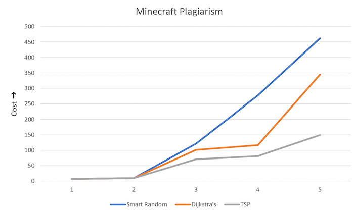
For the really small towers there are not many orders that can be made, so the algorithms work the same. Then, we see a significant drop of the Dijkstra’s and Nearest Neighbor algorithms compared to the smart random algorithm. Then, the Dijkstra’s algorithm stops being a significant improvement compared to the smart random algorithm, and Nearest Neighbor is signficantly better than the other two for the largest structures.
References
https://github.com/topics/travelling-salesman-problem?l=python